Part 2: Calibration and imaging of J1849+3024

This page expects that you have completed part 1 to get as far as applying the Tsys/gain curve, initial delay and bandpass corrections to all sources and split out 1848+283_J1849+3024.ms (and also to become familiar with the basics of CASA).

A new MS contains just a ‘data’ column. The previous applycal made a copy of the data with calibration applied, writing a ‘corrected’ column into the MS and split then took just that column and wrote new data sets, where this becomes a ‘data’ column.

If you don’t have a good version of 1848+283_J1849+3024.ms (remove any bad versions), get 1848+283_J1849+3024.ms.tgz and extract it using tar -zxvf 1848+283_J1849+3024.ms.tgz.

To summarise you will need the following for this part:

1848+283_J1849+3024.ms you made at the end of the initial calibration (end of part 1)
or, 1848+283_J1849+3024.ms.tgz (ready made)
NME_J1849.py included in NME_DARA.tgz from part1

1848+283_J1849+3024.ms contains phase-ref 1848+283 and target J1849+3024. You should have 1848+283_J1849+3024.ms.listobs made at the end of CASA_Basic_EVN which shows the interleaving of the target and phase-ref.

23:20.0 - 13:24:20.0    38      1 1848+283                 18720  [0,1,2,3,4,5,6,7]  [2, 2, 2, 2, 2, 2, 2, 2]
25:00.0 - 13:26:00.0    39      0 J1849+3024               18720  [0,1,2,3,4,5,6,7]  [2, 2, 2, 2, 2, 2, 2, 2]
26:40.0 - 13:27:40.0    40      1 1848+283                 18720  [0,1,2,3,4,5,6,7]  [2, 2, 2, 2, 2, 2, 2, 2]
28:20.0 - 13:29:20.0    41      0 J1849+3024               15840  [0,1,2,3,4,5,6,7]  [2, 2, 2, 2, 2, 2, 2, 2]
30:00.0 - 13:31:00.0    42      1 1848+283                 15840  [0,1,2,3,4,5,6,7]  [2, 2, 2, 2, 2, 2, 2, 2]
...

Preliminary steps & Outline

Before we start:

Look at the script in a text editor (e.g. gedit).

Important: Each step contains one or a few tasks which perform a step in calibration or imaging. It is not completely automatic because it expects interactive imaging, and you need to inspect some of the plots to check and/or to make decisions. The source names and some other parameters are set as variables so the script could be used as a template for other similar data reduction. The taskname(parameter=value) way of running a task automatically sets all unspecified parameters to default. Use inp task or help task at the CASA prompt to check before running a task.

The following calibration script will go through the following (note that the steps correspond to the NME_J1849.py script):

Initial inspection of data (step 1)
Calibration using the phase-reference source
- Time-dependent delay and phase calibration (step 2)
Apply phase solutions and image phase-ref (step 3)
Imaging and self-calibration of the target

1. Initial inspection of data (step 1)

« back to top

# In CASA

mysteps=[1]
execfile('NME_J1849.py')

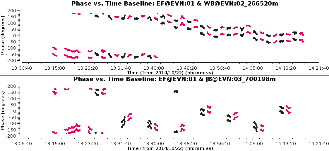
Page through the plots. The phase-ref is in red, target in black. The phase offsets for both sources follow a similar pattern per baseline and correlation, so the phase-reference solutions should also correct the target OK. Note that JB misses every other pair of scans.

2. Calibration using the phase-reference source

a. Time-dependent delay and phase calibration (step 2)

« back to top

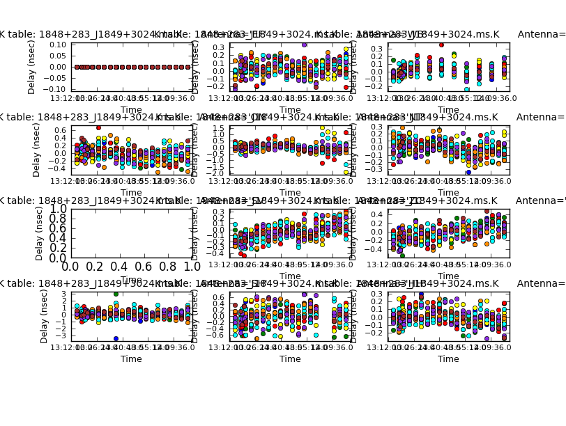
First, we solve for residual delay errors for each scan on the phase-ref.

Set mysteps=[2] and repeat as above and look at the plot of the solutions.

Normally, the bandpass and phase calibrators are different sources; since in this case they are the same, the corrections are very small.

This step also solves for phase as a function of time, averaging all channels (with the new delay corrections applied).

There are a number of considerations in choosing the solution interval. Here, the phase errors do not change massively in a minute, but the S/N is high. So using 30s, half the scan length, means that all the data will be used in interpolating over the target.

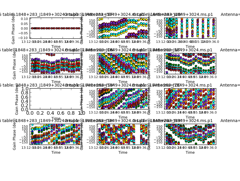
Each colour is a different spw. The phase corrections change more rapidly with time for the antennas on the longest baselines but if you zoom in you can see that the solutions are coherent, not just noise.

2. Apply phase solutions and image phase-ref (step 3)

« back to top

In VLBI, even calibration sources are often resolved (i.e. the source is not a single blob which is the size of the resolution of your array), and so by making an image is also a useful check.

In mystep=[3] we will:

First, the delay and phase corrections are applied to the MS to make a corrected column using applycal.
An initial image of the phase calibrator using the task clean is made to see whether the calibrator is resolved.

The task clean (which always used the corrected data column if it is present) is used for imaging. THe following notes try to decompose the steps clean takes to make you beautiful radio image.

It makes a Fourier Transform (FT) of the visibility data to make what we call the ‘dirty image’, and also makes an FT of the uv coverage to make a ‘dirty beam’ or ‘point spread function’ (psf). The psf often has many sidelobes.
clean also fits an idealised 2D Gaussian to the central peak of the psf. The full width half maximum (FWHM) of this Gaussian is our effective resolution or restoring beam. Important: The pixel size of these images is a free parameter, but you should make it such that there are at least 3, usually 5 pixels across the synthesised beam (you can characterise a Gaussian function using >3 pixels i.e. Nyquist sampled).
clean then goes through many cycles in which it identifies the brightest pixels and then takes 10% (by default) of the flux density at each of these pixels and records the value/position in a model image. clean calculates the sidelobe (i.e. the model x dirty beam) response for each value/position recorder and subtracts that from the dirty map. This is known as a ‘minor cycle’.
After a certain number of minor cycles, the model image is Fourier transformed and subtracted from the visibility data, which are then re-FT’d back to make a new dirty image, which will have less bright emission and fewer sidelobes. This is known as a ‘major cycle’.
These cycles are continued (i.e. steps 3 & 4) until the final dirty image (what we call the ‘residual image’) is indistinguishable from the noise. The model image is then restored to the visibility data (without their sidelobes!), and the result is FT’d and this is convolved with the restoring beam to make the ‘clean image’ (i.e. the one you’d do science with).

You can set a mask to restrict the area of the map in which clean looks for CC, based on inspection and/or prior knowledge of the source.

You can roughly predict the synthesised beam size $\theta_B$ by looking at the antenna positions,

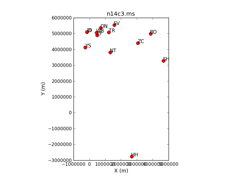
The max. baseline max_B is roughly 10,000 km, and we are observing at 5 GHz, so (all in metres):

max_B = 10000000.
wavelength = 0.06
theta_B= 3600.*degrees(wavelength/max_B)   # convert from radians to degrees and thence to arcsec
theta_B

You can just cut-and-paste this into CASA which returns theta_B ~ 0.001 arcsec = 1 mas. 0.0002 arcsec is thus a good pixel size. The overall image size is determined by how large you think the source is (here we assume that a phase-reference is compact) or the field of view, and this image size must be even (a power of 2 or multiples of 2,3,5,7 are fast).

Here is an explanation of the relevant parameters:

os.system('rm -rf '+phscal2+'_phasecal.clean*')   # delete any failed attempts
clean(vis=phscal2+'_'+target2+'.ms',
      imagename=phscal2+'_phasecal.clean',
      field=phscal2,
      imsize=256,                        # Image size ~50 mas should be big enough
      cell='0.0002arcsec',               # Pixel size calculated above
      niter=100,                         # Total number of clean iterations
      cyclefactor=1,                     # Speed up clean with a higher ratio minor:major cycles, OK for a compact source.
      interactive=True,                     # Set/change mask manually
      npercycle=50,                      # Return partly-cleaned image for inspection/changing mask every 50 iterations
      usescratch=True)                      # Write model to MS for use in calibration

Run mystep=[3] - we will demonstrate how to set the mask.

If you make a mess, you can type execfile('clean.last') to restore the inputs and change what you need; don’t forget to delete the failed attempt first. Or just cut and paste from above, if you just messed up masking.

# In CASA
!ls -d *_phasecal.clean*

which shows:

1848+283_phasecal.clean.flux/          # Primary beam response (in CASAv4)
1848+283_phasecal.clean.pb/          # Primary beam response (in CASAv5+)
1848+283_phasecal.clean.image/         # Clean image
1848+283_phasecal.clean.mask/          # The mask you used
1848+283_phasecal.clean.model/         # The CC
1848+283_phasecal.clean.psf/           # Dirty (synthesised) beam
1848+283_phasecal.clean.residual/      # Residual before restoring CC

Inspect the clean image using the CASA viewer:

# In CASA
viewer('1848+283_phasecal.clean.image')

You can change the display interactively, load the dirty beam etc.

The script also reports the image rms, peak and S/N. I got a peak brightness of 1.292 Jy/bm, rms 0.040 Jy/bm, S/N 32. You may get different numbers depending on how you set the mask and how many iterations you did, but they should be similar.

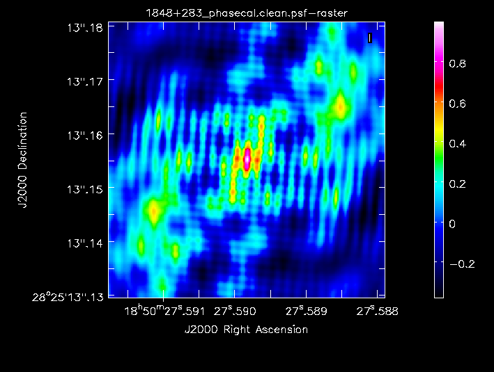
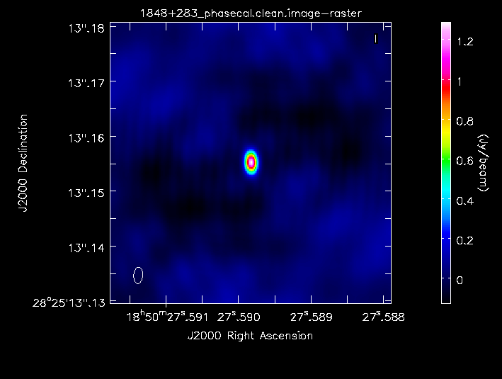
a. Check for remaining bad data (step 4)

« back to top

If this was a data set no-one had looked at before, you would inspect the data manually, not in the script, in order to page through all the baselines and identify bad data, but it is not the best use of your time here, so all the flagging was already applied.

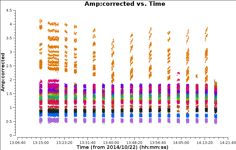
Just run mysteps=[4] to check. This plot shows all the baselines to EF on one plot:

b. Time-dependent amplitude calibration (step 5)

« back to top

Whilst the application of Tsys (early in the data reduction) should scale the amplitudes, it is subject to instrumental error and the previous plot shows at least one antenna with suspiciously high amplitudes. This limits the S/N that we imaged before therefore to improve this we do amplitude calibration on the phase calibrator to improve the Tsys amplitude estimates.

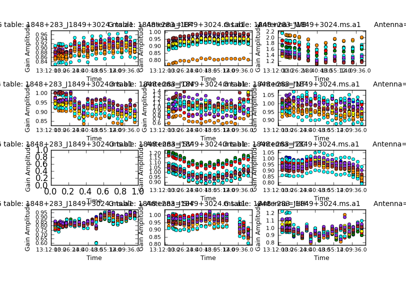
To do this, inspect mysteps=[5] and run it.

solnorm=True means, estimate the corrections with one solution per solution interval & antenna & polarisation. Then form the mean product of all the amplitude solutions and divide each solution by this. This means that the relative variations of the solutions with time etc. are corrected, but the product of the gains overall is unity so an image made from the data will still have the same flux scale. CASA gain solutions are divided into the data, so a high gain will correct a high amplitude, as seen for the second antenna.

c. Apply amplitude and phase solutions to the phase-ref (step 6)

« back to top

Run mysteps=[6] to apply the solutions and inspect the corrected data.

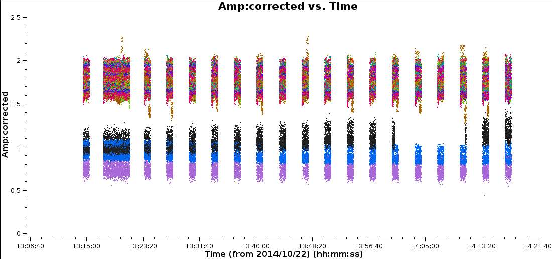
This plot shows only baselines to EF. There is now less scatter but there are two groups of baselines with quite distinct flux densities. However, this could be due to the source being resolved.

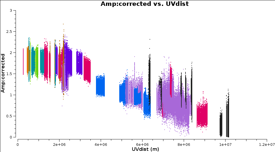
Plotting amplitude against uv distance (for all baselines) shows that indeed there is more flux on short baselines than on long baselines i.e. the source is resolved (if it was unresolved then the flux should be the same on ALL fourier/uv scales!)

d. Clean the calibrated phase-ref (step 7)

« back to top

As before, mysteps=[7] needs you to set a mask interactively.

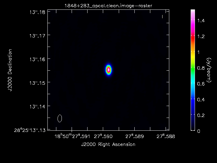
After cleaning, I got a peak brightness 1.529 Jy/bm, rms 0.001 Jy/bm, S/N 1599 - a big improvement!

e. Uncalibrated target image (step 8)

« back to top

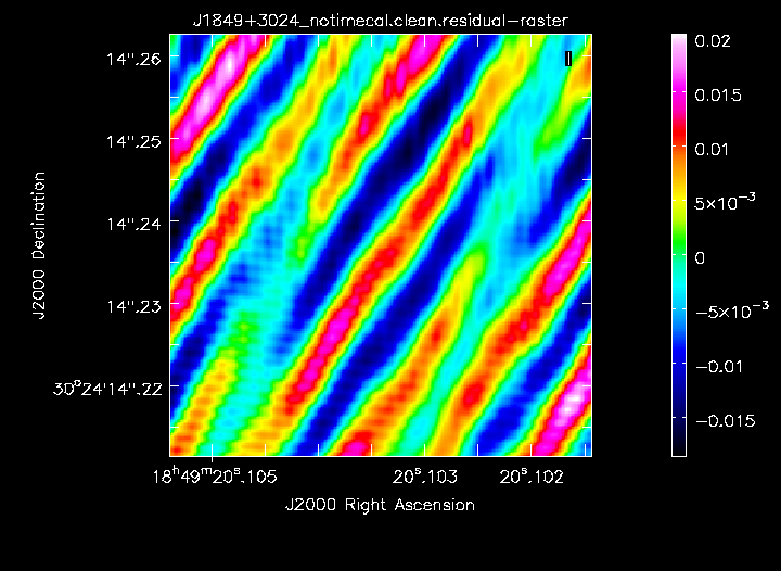
So far, we have applied the Tsys and gain-elevation curve corrections to the amplitudes for all data, and we have applied the initial delay and bandpass corrections to all data. This phase-ref has also had more calibration applied but we have not yet applied any time-dependent calibration of phase to the target. To illustrate that we require time-dependent calibration we shall image the target without these applied! (This is not a normal step as it is useless, this is just for demonstration)

Run mystep=[8] - this does not do any cleaning because one look at the dirty image shows that it is useless.

f. Apply all calibration to the target (step 9)

« back to top

Run mystep=[9]

The phase reference solutions are now interpolated over the target data. Since the data are taken close in time and the sources are close together on the sky, we assume that the atmospheric distortions are similar. In the plot you made above, in ‘Check for remaining bad data (step 4)’ you see that one antenna only records every other pair of target - phase-ref scans. This is JB, and in order to allow for the longer gaps, we handle it separately (this may not always be necessary in future versions of CASA).

In the first applycal all the antennas except JB are corrected. CASA task smoothcal then is used to smooth the JB solutions over an interval longer than the gaps between its pairs of scans, for each table, and then the smoothed table is applied to JB only. Parameter interp=['nearest','nearest','nearest'] has three values because we are applying 3 calibration tables. (The default is linear for linear interpolation but this can miss data if the final phase-ref scan is missing and extrapolation is needed instead).

4. Imaging and self-calibration of the target

a. Split out target 2 and image (step 10)

« back to top

Run mystep=[10] and clean interactively.

Important From now on, the input MS is J1849+3024.ms

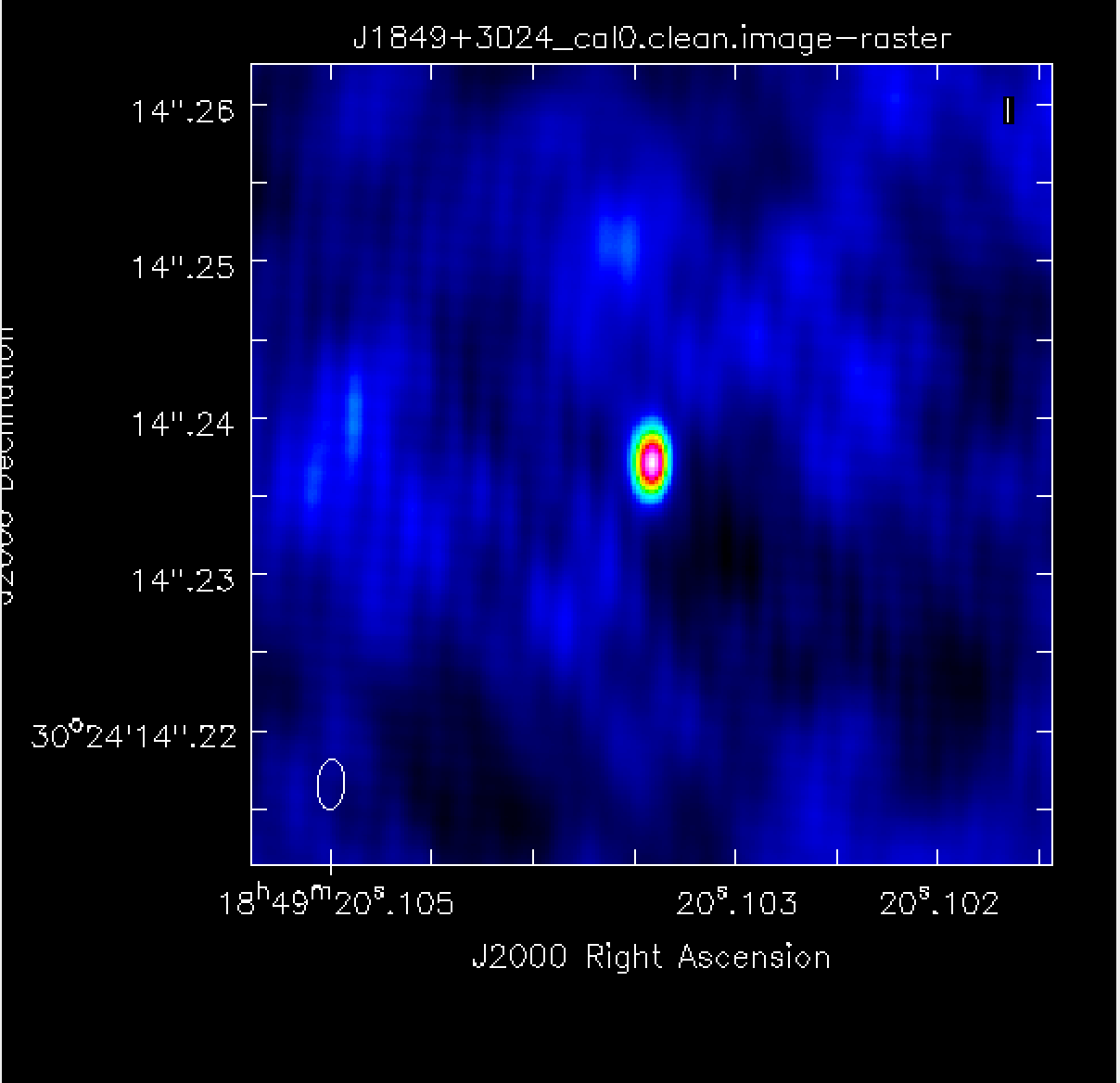
I got Peak 0.211, rms 0.010, S/N 21

This is not as low noise as the final phase-ref image because the separation on the sky and in time is enough for there to be small differences in atmosphere. These are corrected by self-calibration. This is the same principle as we used above using the phase reference source to derive corrections, except that in this case we only apply the corrections to the same source, the target itself. Also, in the very first round of calibration, the model is the CC made from the image we just made after applying the phase-reference solutions, i.e. it is already a good approximation to the actual structure and position of the target (without depending on a catalogue value).

This map shows dominantly asymmetric artefacts (positive on one side of the source, negative on the other) which are due to remaining phase errors.

Self-calibrate target phase only and apply (step 11)

« back to top

Later in the week we will discuss in more detail why a solution interval of 10 sec is used. Empirically, you see that only a few solutions fail, and it is short enough to give accurate corrections. The plot below shows that there are quite large residual corrections for some antennas, but they have structure, not just noise.

Run mysteps=[11]

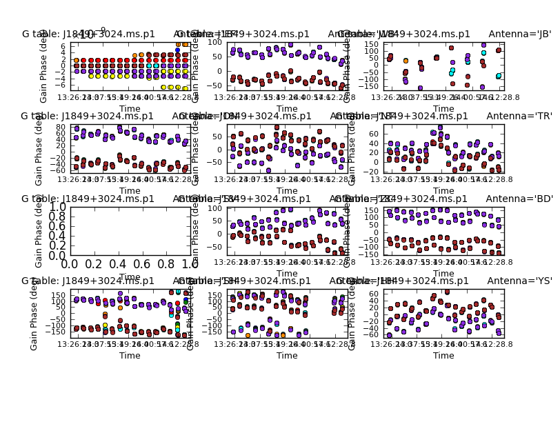
Image phase self-calibrated target (step 12)

« back to top

Run mysteps=[12] with interactive cleaning.

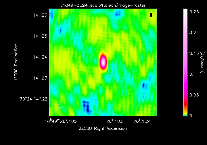
I got peak of 0.256 Jy/bm, rms 0.001 Jy/bm, S/N 249 so a nice improvement.

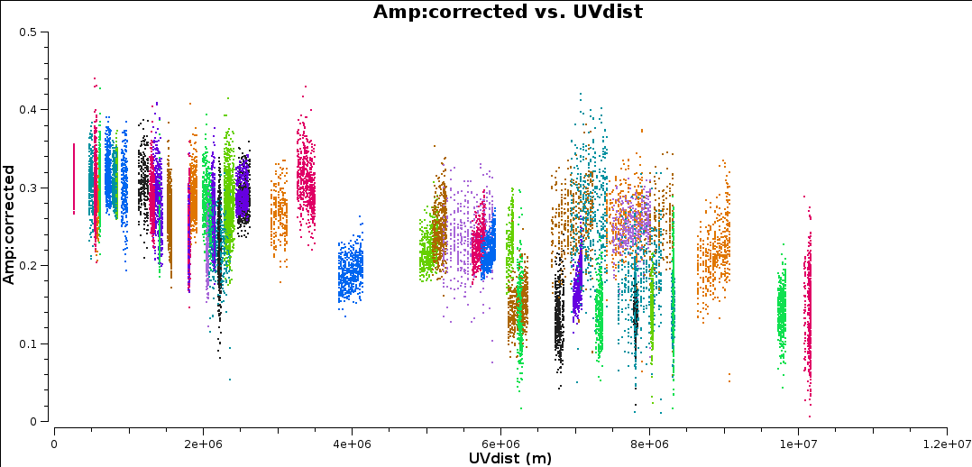
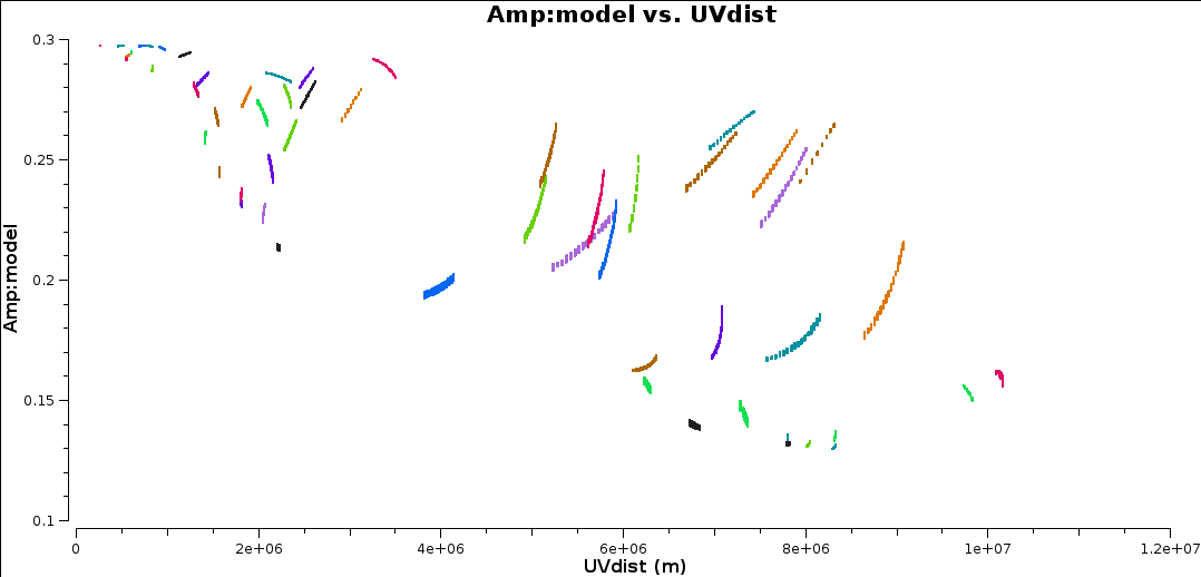
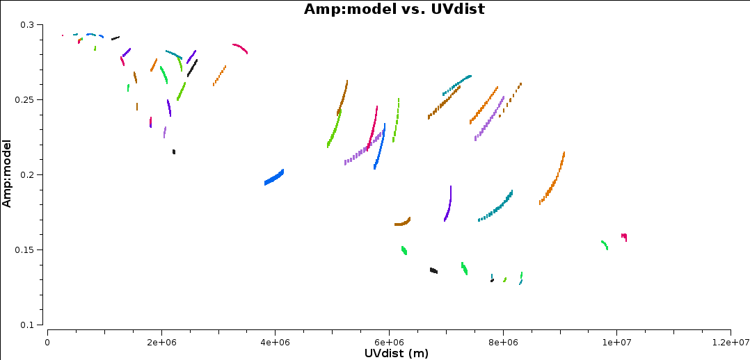
This step plots the corrected data and the model uv amplitudes, colourised by baseline. You can see that although the data have more scatter, the model does represent the data quite well, i.e. the CC have been located where there is real emission, not sidelobes, and the image has not missed bright emission.

Self-calibrate target amplitude and phase and apply (step 13)

« back to top

Run mysteps=[13].

The amplitude errors change more slowly than phase errors and as we are applying the phase solutions we can average for longer in time to get better S/N. The solutions are mostly close to unity with no very wild ones.

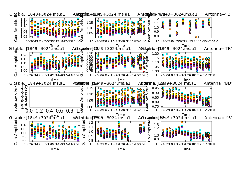
Image the amplitude and phase self-calibrated target (step 14)

« back to top

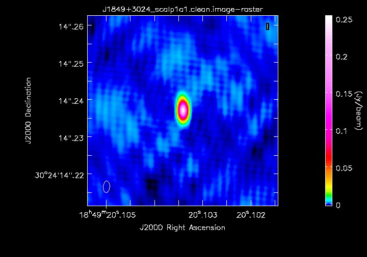
Run mysteps=[14] with interactive cleaning.

I got peak of 0.254 Jy/bm, rms 0.001 Jy/bm, S/N 311 so the noise is as good as for the phase-ref.

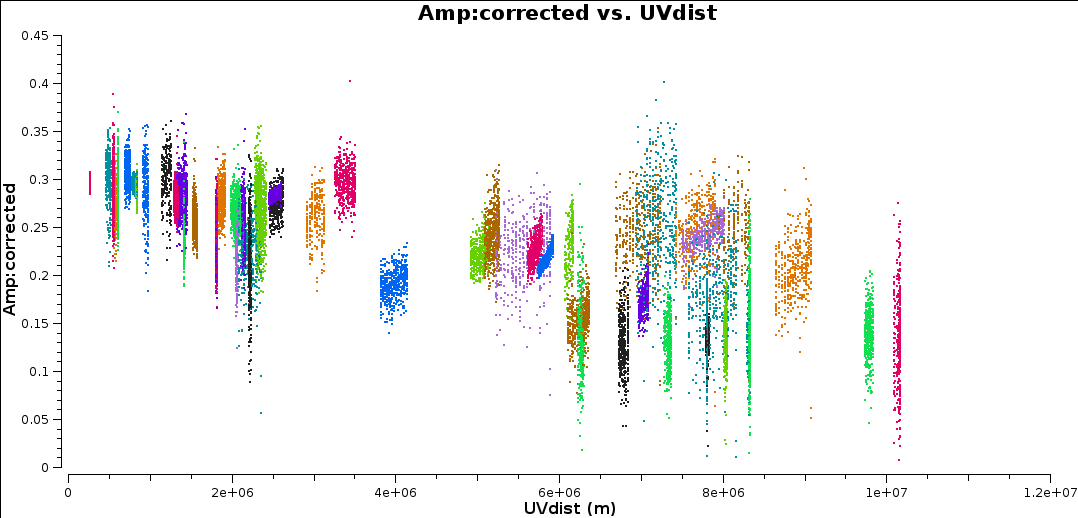
The differences between the uv plots of these averaged data before and after the final calibration are hard to see, but enough to make the improvement in S/N.

Congralulations! You have finished imaging J1849+3024. Now onto part3!

Development-in-Africa-Unit-4