Part 1: CASA Basic EVN Calibration
« Return to homepage
« Return to EVN continuum
Guidance for calibrating EVN data using CASA
This guide uses capabilities of CASA 4.7.2; CASA 5+ does work apart from the Tsys calibration step (and the script isn’t fixed yet, see Issue #1).
It is suitable for good-quality EVN data which does not require the use of ‘rate’ in calibration. It also requires a prepared gaincurve table and helper scripts if you are starting from the fitsidi data. You need about 20 G disk space, although one could manage with less by moving early versions of these files to storage.
This section is organised as follows:
- Data and supporting material
- How to use this guide
- Data loading and inspection
- Frequency-related calibration
- Apply calibration and split out phase-ref - target pairs
1. Data and supporting material
n14c3 is an EVN network monitoring experiment. It contains two target - phase-reference pairs of bright sources (plus a 5th source which we will not use). The full data reduction here needs:
- Raw data (fits IDI files from the JIVE correlator)
- n14c3_1_1.IDI1,
- n14c3_1_1.IDI2
- Gain curve and Tsys tables (specially prepared for this data set by Mark Kettenis and Anita Richards)
- n14c3.gc
- n14c3.antab
- Helper scripts by Mark Kettenis to convert the .antab Tsys table to the correct format
- key.py
- tsys_spectrum.py
- Flag command files. You can write these yourself but to save time you can use some or all of these
- flagSH.flagcmd
- flagSH1.flagcmd
- flagTar1Ph1.flagcmd
These are all provided on your desktop for the DARA workshops, but the fits IDI files can also be obtained from here along with more information about the observations. The other files are available in the tar file: NME_DARA.tgz
- List of data reduction scripts and intermediate data products for each part
- Part1: Initial data inspection and calibration common to all sources: files listed above. Optional NME_all.py is a script version of the commands, for your future reference.
- Part2: Further calibration and imaging of 1848+283/J1849+3024.
- 1848+283_J1849+3024.ms you made at the end of the initial calibration (end of part 1)
- or, 1848+283_J1849+3024.ms.tgz (ready made)
- NME_J1849.py
- Part3: Further calibration and imaging of J1640+3946/3C345.
- J1640+3946_3C345.ms you made at the end of the initial calibration (end of Part 1)
- or, J1640+3946_3C345.ms.tgz (ready made);
- NME_3C345_skeleton.py
- (NME_3C345.py.gz is complete script for future reference)
These are the sources:
| Number | Name | Position (J2000) | Role |
|---|---|---|---|
| 0 | J1640+3946 | 16:40:29.632770 +39.46.46.02836 | target |
| 1 | 3C345 | 16:42:58.809965 +39.48.36.99402 | phase-cal |
| 2 | J1849+3024 | 18:49:20.103406 +30.24.14.23712 | target |
| 3 | 1848+283 | 18:50:27.589825 +28.25.13.15523 | phase-cal |
| 4 | 2023+336 | 20:25:10.842114 +33.43.00.21435 | not used |
J1849+3024 is also used as bandpass calibrator because it is a bright, compact source with good data on all baselines. If you are reducing a new data set, you would check the suitability of the bandpass calibrator during early data reduction.
2. How to use this guide
This web page presents inputs for CASA tasks to be entered interactively at a terminal prompt for the calibration of the averaged data and initial target imaging. This is useful to examine your options and see how to check for syntax errors.
- To begin with, work interactively to see what each parameter is for. This is used for the initial steps and calibration common to all sources.
- Calibrate and image one phase-reference and target using a script (
NME_J1849.py). - Use this information to enter parameters and values in
NME_3C345_skeleton.pyfor the other phase-ref - target pair.
To start:
- Make a directory called something you will remember, e.g. EVN, and work in it. (Do not do data reduction within the CASA installation).
- Copy the data and files you need to this directory. <path***> is the original location of these files; Note in general, *** means something for you to fill in. e.g:
mdir EVN
cd EVN
cp <path***>/n14c3_1_1.IDI? .
cp <path***>/NME_DARA.tgz .
cp <path***>/*py .

tar -zxvf NME_DARA.tgz          # extract the additional material (also the scripts  which will be supplied).
3. Data loading and inspection
- Check that you are in the right place with all the data.
pwd                   # tells you present working directory
ls
which should show

flagSH1.flagcmd      key.py          n14c3.antab        NME_3C345_skeleton.py  NME_J1849.py
flagSH.flagcmd       n14c3_1_1.IDI1  n14c3.gc           NME_all.py             tsys_spectrum.py
flagTar1Ph1.flagcmd  n14c3_1_1.IDI2  NME_3C345.py       NME_DARA.tgz
- Now start CASA.
a. Load data and correct for Earth rotation
- The first task is
importfitsidiwhich converts the fits files to CASA-amicable Measurement Sets (MS). Copy these lines one at a time (when you get more familiar, some inputs can be copied together).
# in CASA
os.system('rm -rf n14c3_prefix.ms*')              # make sure no old files are present

default(importfitsidi)                            # initialise task
inp()                                             # list all inputs

fitsidifile=['n14c3_1_1.IDI1','n14c3_1_1.IDI2']   # fits files to convert
vis='n14c3_prefix.ms'                            # output ms file name
constobsid=True                                   # data could be processed together
scanreindexgap_s=15                               # only separate scans if gap >15 sec (or source change)
inp()                                             # check your inputs

importfitsidi()                                   # if happy, execute the task
inp() provide checks that you should normally carry out but the script won’t repeat these for every task.
Note A few warnings about DIAMETER and POLCALA/B and zero/negative scan Nos may appear because CASA is not yet fully adapted for VLBI data but normally can be ignored if the task finishes ok. Check you CASA logger just in case.
Important You can review the inputs to the last time you ran a task by typing:
# In CASA:
ls      # This should show the MS you just created and importfitsidi.last

!more importfitsidi.last   # ! allows you to run any linux shell command
This will show something like:

taskname           = 'importfitsidi'
fitsidifile        =  ['n14c3_1_1.IDI1', 'n14c3_1_1.IDI2']
vis                =  'n14c3__prefix.ms'
constobsid         =  True
scanreindexgap_s    =  15
#importfitsidi(fitsidifile=['n14c3_1_1.IDI1', 'n14c3_1_1.IDI2'],vis="n14c3__prefix.ms",constobsid=True,scanreindexgap_s=15)
The first format is for the interactive input (i.e. what you type directly into CASA), and the second format (without ‘#’) is for use when scripting (automatic calibration! woo!).
- Now adjust the uvw coordinates to allow for the projection effect as the Earth rotates.
# In CASA:
os.system('rm -rf n14c3.ms')
os.system('rm -rf n14c3.ms.flagversions')

default(fixvis)
vis='n14c3_prefix.ms'
outputvis='n14c3.ms'

fixvis()
- List the contents of the measurement set (creates a new file called
n14c3.ms.listobsin your current directory)
# In CASA:
os.system('rm -rf n14c3.ms.listobs')

default(listobs)
vis='n14c3.ms'
listfile='n14c3.ms.listobs'
listobs()
- Inspect this listing in
gediti.e. type in CASA!gedit n14c3.ms.listobsor use a text viewer of your choice.
Important The listobs output give information on what is contained in your data set i.e. antennas, sources, scans etc. The following section breaks this file down:
- Scan listing: this shows the pattern of observations. Each scan is about 1 min and each individual integration about 2 sec.
Date Timerange (UTC) Scan FldId FieldName nRows SpwIds Average Interval(s) ScanIntent 22-Oct-2014/12:00:00.0 - 12:04:00.0 1 1 3C345 52800 [0,1,2,3,4,5,6,7] [2, 2, 2, 2, 2, 2, 2, 2] 12:06:00.0 - 12:10:00.0 2 1 3C345 63360 [0,1,2,3,4,5,6,7] [2, 2, 2, 2, 2, 2, 2, 2] 12:12:00.0 - 12:13:00.0 3 1 3C345 15840 [0,1,2,3,4,5,6,7] [2, 2, 2, 2, 2, 2, 2, 2] 12:13:40.0 - 12:14:40.0 4 1 3C345 15840 [0,1,2,3,4,5,6,7] [2, 2, 2, 2, 2, 2, 2, 2] 12:15:20.0 - 12:16:20.0 5 0 J1640+3946 15840 [0,1,2,3,4,5,6,7] [2, 2, 2, 2, 2, 2, 2, 2] 12:17:00.0 - 12:18:00.0 6 1 3C345 13200 [0,1,2,3,4,5,6,7] [2, 2, 2, 2, 2, 2, 2, 2] 12:18:40.0 - 12:19:40.0 7 0 J1640+3946 13200 [0,1,2,3,4,5,6,7] [2, 2, 2, 2, 2, 2, 2, 2] ... - Names and positions of fields observed.
Fields: 5 ID Code Name RA Decl Epoch nRows 0 J1640+3946 16:40:29.632770 +39.46.46.02836 J2000 254400 1 3C345 16:42:58.809965 +39.48.36.99402 J2000 383520 2 J1849+3024 18:49:20.103406 +30.24.14.23712 J2000 276480 3 1848+283 18:50:27.589825 +28.25.13.15523 J2000 388800 4 2023+336 20:25:10.842114 +33.43.00.21435 J2000 542880 - Correlator set-up: there are 8 spectral windows (AKA IFs), each of 32 channels, and 4 polarization products (we will only use the total intensity combination of RR and LL).
Spectral Windows: (8 unique spectral windows and 1 unique polarization setups) SpwID Name #Chans Frame Ch0(MHz) ChanWid(kHz) TotBW(kHz) CtrFreq(MHz) Corrs 0 none 32 TOPO 4926.990 500.000 16000.0 4934.7400 RR RL LR LL 1 none 32 TOPO 4942.490 500.000 16000.0 4950.2400 RR RL LR LL 2 none 32 TOPO 4958.990 500.000 16000.0 4966.7400 RR RL LR LL 3 none 32 TOPO 4974.490 500.000 16000.0 4982.2400 RR RL LR LL 4 none 32 TOPO 4990.990 500.000 16000.0 4998.7400 RR RL LR LL 5 none 32 TOPO 5006.490 500.000 16000.0 5014.2400 RR RL LR LL 6 none 32 TOPO 5022.990 500.000 16000.0 5030.7400 RR RL LR LL 7 none 32 TOPO 5038.490 500.000 16000.0 5046.2400 RR RL LR LL - Antennas used. The Offset from array center is zero since the absolute Earth-centred coordinates are given for each antenna.
Antennas: 12:
  ID   Name  Station   Diam.    Long.         Lat.                Offset from array center (m)                ITRF Geocentric coordinates (m)
                                                                 East         North     Elevation               x               y               z
  0    EF    EVN:01    0.0  m   +006.53.01.0  +50.20.09.1          0.0000        0.0000  6365855.3595  4033947.234200   486990.818800  4900431.012900
  1    WB    EVN:02    0.0  m   +006.38.00.0  +52.43.48.0          0.0000        0.0000  6364640.6582  3828445.418100   445223.903400  5064921.723400
  2    JB    EVN:03    0.0  m   -002.18.30.9  +53.03.06.6         -0.0000        0.0000  6364633.4245  3822625.831700  -154105.346600  5086486.205800
  3    ON    EVN:04    0.0  m   +011.55.04.0  +57.13.05.3          0.0000        0.0000  6363057.6347  3370965.885800   711466.227900  5349664.219900
...
b. Fix antenna and Tsys tables
These steps may not always be needed as CASA and EVN data formats become more compatible especially with the VLBI tools getting released with CASA v5.3+.
The antab table has to be converted into a subtable within the MS using tsys_spectrum.py. This is then be used to generated a Tsys correction table using gencal. The system temperature is measured every few minutes. This compensates roughly for the different levels of signal from different sources, the effects of elevation and other amplitude fluctuations. Each antenna has a characteristic response in terms of Kelvin of system temperature per Jy of flux, so Tsys is also used to scale the flux density.
# In CASA:
inbase='n14c3'                   # pass base name to script
execfile('tsys_spectrum.py')     # execfile runs any suitable script inside CASA

os.system('rm -rf n14c3.tsys')

default(gencal)  # This reads the Tsys information we just wrote into the MS and derives a calibration table
vis='n14c3.ms'
caltable='n14c3.tsys'
caltype='tsys'

gencal()
Plot the table generated.
# In CASA:
default(plotcal)
caltable='n14c3.tsys'
xaxis='freq'
yaxis='tsys'
subplot=431
iteration='antenna'
plotcal()
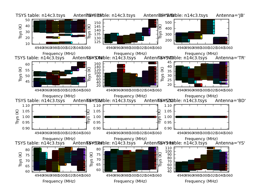
You can see the changes with each source change.
Three antennas do not have Tsys measurements but the .gc (gain curve) table provides a scaled gain-elevation correction which scales the visibility amplitudes, although without any allowance for weather or source contribution
listobs gave the antenna diameters as zero since the information is not written into the fits files for EVN data. Some antennas have off-axis feeds and so the offsets also have to be inserted.
# In CASA
# Copy these arrays of values (no line breaks in each array)
ants=  ['EF','WB','JB','ON','NT','TR','SV','ZC','BD','SH','HH','YS','JD']
diams= [100.0,300.0,75.0,25.0,32.0,32.0,32.0,32.0,32.0,25.0,24.0,40.0,25.0]
axoffs=[[0.013,4.95,0.,2.15,1.831,0.,-0.007,-0.008,-0.004,-0.002,6.692,2.005,0.]
        ,[0.,0.,0.,0.,0.,0.,0.,0.,0.,0.,0.,0.,0.]
        ,[0.,0.,0.,0.,0.,0.,0.,0.,0.,0.,0.,0.,0.]]

# Modify the antenna table
tb.open('n14c3.ms/ANTENNA', nomodify=F)
tb.putcol('DISH_DIAMETER', diams)
tb.putcol('OFFSET',axoffs)
tb.close()

default(listobs)     # Check in listobs
vis='n14c3.ms'
listobs()
This time we don’t write a text file because the parameter listfile was not set, so just look in the logger to ensure that the antenna diameters now appear.
c. Inspect and flag data
- Lets first flag the autocorrelations for continuum data (ignore warnings about the processor).
# In CASA
default(flagdata)
vis='n14c3.ms'
mode='manual'
autocorr=T

flagdata()
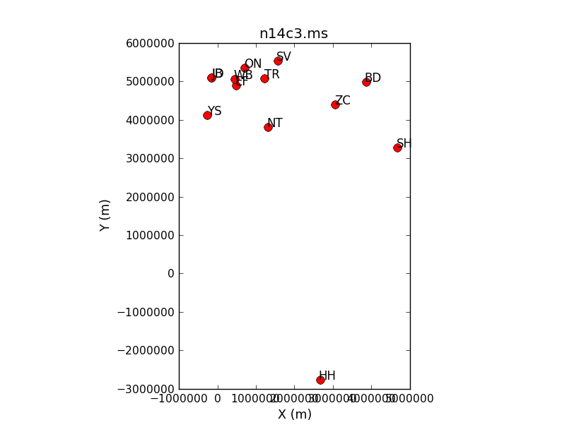
- Next: lets plot the location of antennas using task
plotants.
# In CASA
default(plotants)
vis='n14c3.ms'

plotants()
- Now we shall use
plotmsto plot the visibility data. We start by looking at a bright source where it is easiest to tell good and bad data apart.
# In CASA
default(plotms)
vis='n14c3.ms'
xaxis='frequency'
yaxis='amp'
field='1848+283'        # The phase-cal/bandpass cal
avgtime='3600'          # Will only average within scans unless additionally told to average scans too
antenna='EF&*'          # Plot all baselines to the largest and most sensitive antenna
correlation='RR,LL'     # Only plot the parallel hands; the cross hands are fainter (and we won't be using them).
coloraxis='antenna2'

plotms()
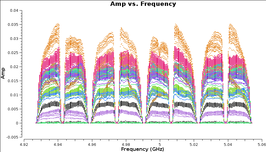
- You can change the plot interactively in plotms.
- You can see 8 spw; the edges of this have low amplitudes due to poor sensitivity and there are some data all at zero.
- Zoom in (using
 ) and use select to highlight bad data (
 ) and use locate (
 ) to see what antenna it is associated with.
 -
You should find that this is mostly SV (dark green in this plot).
- Important: Before more flagging, remember to back up the current flags. Do this any time you think you might need to change your mind about flagging; use a different version name each time and make a note of it (CASA task
flagdatacan make an automatic backup but it will not have a memorable name). The backups for this data set are stored inn14c3.ms.flagversions.We will now back up the flags for this data set now:
  # In CASA
  default(flagmanager)
  vis='n14c3.ms'
  mode='save'
  versionname='preSVandEndChans'

  flagmanager()
- After identifying the bad data using
plotmswe can flag antenna SV (only one polarisation is bad but CASA can’t yet calibrate a single polarisation so we need to remove the whole antenna).
  # In CASA
  default(flagdata)
  vis='n14c3.ms'
  mode='manual'
  antenna='SV'
- Now we should re-inspect the data for any more corrupted data. Plot the most sensitive baseline to see the end channels more clearly and note which are below about half the maximum amplitude.
# In CASA
default(plotms)
vis='n14c3.ms'
xaxis='channel'
yaxis='amp'
field='1848+283'        # The phase-cal/bandpass cal
avgtime='3600'          # Will only average within scans unless additionally told to average scans too
antenna='EF&JB'          # Plot all baselines to the largest and most sensitive antenna
correlation='RR,LL'     # Only plot the parallel hands; the cross hands are fainter (and we won't be using them).
iteraxis='spw'

plotms()
- Use the arrows at the bottom of
plotmsto scroll through the spw. Odd and even spw behave differently but there is no need to spend too much time on this as the suggested channels to flag are given here for time saving purposes:
# In CASA
default(flagdata)
vis='n14c3.ms'
mode='manual'
spw='0:0~5;29~31,2:0~5;29~31,4:0~5;29~31,6:0~5;29~31,1:0~2;27~31,3:0~2;27~31,5:0~2;27~31,7:0~2;27~31')

flagdata()
- Reinspect again and plot amp v. time, now averaging in frequency not time:
# In CASA
default(plotms)
vis='n14c3.ms'
xaxis='time'
yaxis='amp'
field='1848+283'
spw='0~7:13~20'        # Average a few central channels where the response is stable
avgchannel='8'
antenna='EF&*'
correlation='RR,LL'
coloraxis='baseline'

plotms()
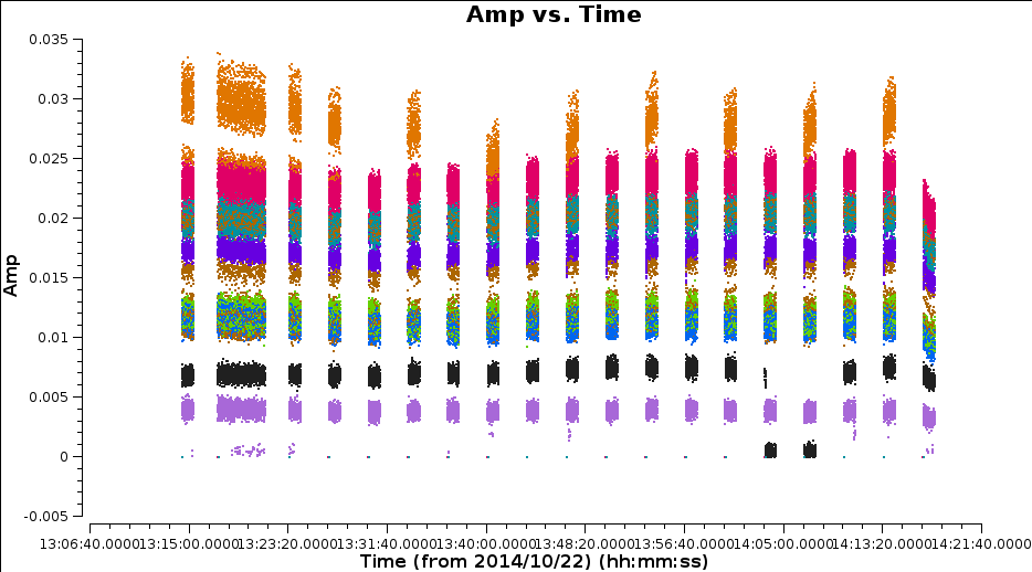
- Note that the first one or two integrations of each scan are bad. There is a specific
flagdatamode for this calledquack. We will safely assume that all sources are affected.
# In CASA
default(flagdata)
vis='n14c3.ms'
mode='quack'
quackinterval = 5     # 5 seconds, or just over 2 intgrations

flagdata()
- Now go through each baseline to identify remaining bad data (enter
iteration='baseline'and re-loadplotms). Again, this has already been listed so don’t spend too long, just make sure you have some idea of how to identify and record bad data. There is more than one bad scan on HH and as we are plotting the phase-cal it is likely that the target in-between was affected. Plot this.
# In CASA
default(plotms)

vis='n14c3.ms'
xaxis='time'
yaxis='amp'
scan='60~70'            # a few scans including the bad data; plot all fields in this time range
spw='0~7:13~20'
avgchannel='8'
antenna='EF&HH'         # just the relevant baseline
correlation='RR,LL'
coloraxis='field'       # distinguish sources

plotms()
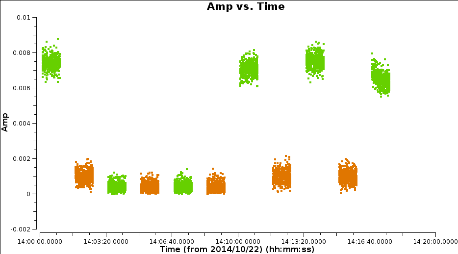
- Flag the scans when the target (in brown in the plot here) goes right to zero.
# In CASA
default(flagdata)
vis='n14c3.ms'
antenna='HH'
mode='manual'
scan='62~65'

flagdata()
- Inspect the next most distant antenna, SH
# In CASA
default(plotms)

vis='n14c3.ms'
xaxis='time'
yaxis='amp'
field='1848+283'
spw='0~7:13~20'
avgchannel='8'
antenna='EF&SH'         # just the relevant baseline
correlation='RR,LL'
coloraxis='spw'         # distinguish spw

plotms()
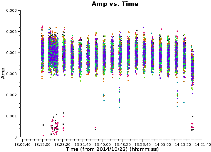
There are many short, bad periods, some only affecting certain spw. The easiest way to cope with this is to write a flag list. Identify antennas/spw/times, adding 1s to the start and finish of each flagging period. They are all shorter than one scan so the same flags aren’t applied to the target but later, we will look for similar bad data on the target. Take a look at the flag list file: flagSH.flagcmd which is in your current directory and cross-check that these entered values are affected.
If you are happy, then we use this file to automatically flag those channels specified in the file:
# In CASA
default(flagdata)
vis='n14c3.ms'
mode='list'
inpfile='flagSH.flagcmd'

flagdata()
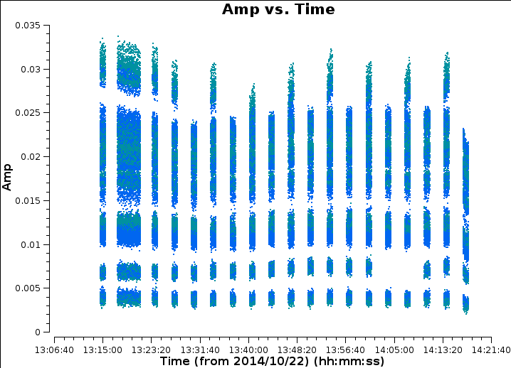
- Reinspect to check that the bad data are all gone:
# In CASA
default(plotms)
vis='n14c3.ms'
xaxis='time'
yaxis='amp'
field='1848+283'
spw='0~7:13~20'
avgchannel='8'
antenna='EF&*'
coloraxis='corr'
correlation='RR,LL'

plotms()
4. Frequency-related calibration
a. Delay calibration
The signal from each VLBI antenna is timestamped in order to allow synchronisation of all antennas when they are correlated. Small clock errors cause a frequency-dependent phase shift in the correlated signal, i.e. a slope of the phase across the band.
- Lets examine this, and we shall average the time within each scan.
# In CASA
default(plotms)
vis='n14c3.ms'
xaxis='freq'
yaxis='phase'
field='1848+283'
avgtime='3600s'
antenna='EF&*'
coloraxis='corr'
iteraxis='baseline'
correlation='RR,LL'

plotms()
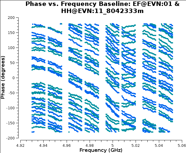
The phases have a random wiggle (which will be corrected later) as well as a systematic slope, which is more or less the same for each scan.
- Lets pick a scan with all spw and antennas present (e.g. for the plot below I chose #38):
# In CASA
default(plotms)
vis='n14c3.ms'
xaxis='scan'
yaxis='amp'
field='1848+283'
spw='0~7:13~20'
avgchannel='8'
avgtime='3600'
antenna='EF&*'
coloraxis='antenna2'
correlation='RR,LL'

plotms()
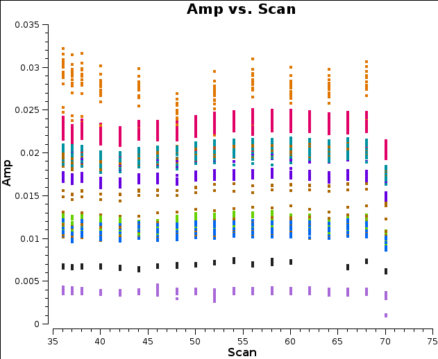
Important: Delay calibration derives the gradient of phase against frequency, which can divided into the complex data to remove the systematic slope.
- In CASA, we can determine this using a bright source, long solution interval (so we only correct in the frequency dimension). The task
gaincaldetermines this solution:
# In CASA
default(gaincal)
vis='n14c3.ms'
caltable='n14c3_bpcal.K'  # File name for output calibration table
field='1848+283'
scan='38'
solint='150s'             # longer that the scan, to make sure just one solution
refant='EF'               # The most sensitive antenna, with many shorter baselines, as the zero of phase.
gaintype='K'              # Solve for delay
parang=T                  # Apply the parallactic angle correction for the feed rotation of Alt-Az telescopes

gaincal()
- And we shall plot this calibration table using
plotcalagain:
default(plotcal)
caltable='n14c3_bpcal.K'
xaxis='freq'
yaxis='delay'
iteration='antenna'
subplot=431

plotcal()
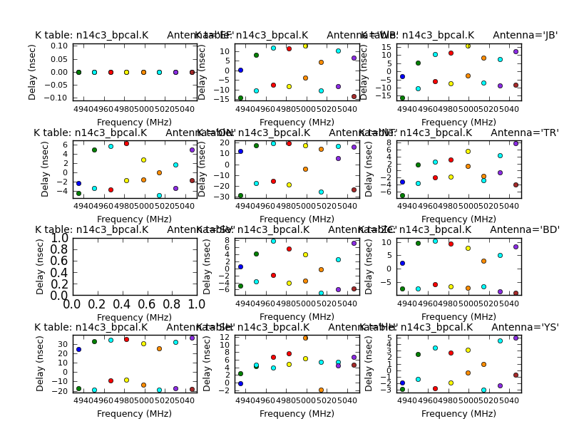
The solutions are smooth in frequency and don’t have massive values (30ns is ok for EVN observations). Note that the delay solutions are proportional to the baseline length (see the plotants image for reference)
b. Pre-bandpass time-dependent phase correction
We need now need to correct channel-by-channel errors but in order to get high enough signal to noise, we need to average the data in time. However, in order to do that, we need to average in time. The delay corrections just derived are good enough to allow preliminary channel averaging to derive time-dependent solutions before doing this.
- Lets first look at phases versus time using
plotmsagain:
# In CASA
default(plotms)
vis='n14c3.ms'
xaxis='time'
yaxis='phase'
field='1848+283'
spw='0~7:13~20'
avgchannel='8'
antenna='EF&*'
coloraxis='spw'
iteraxis='baseline'
correlation='RR'

plotms()
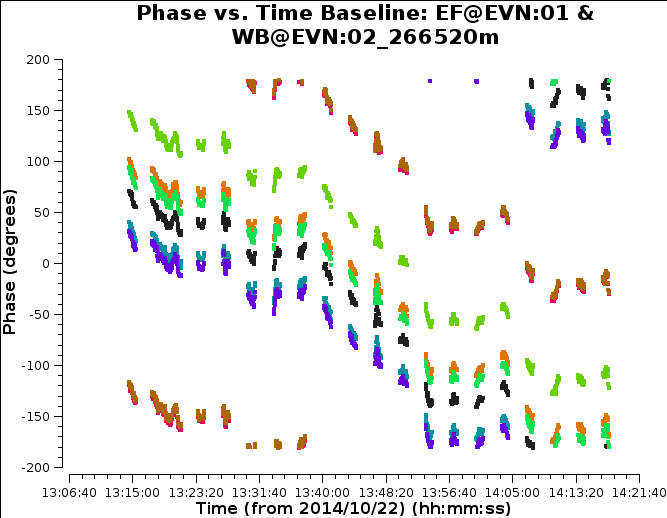
And zooming into a single scan reveals:
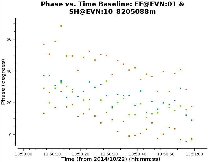
Some notes on these plots:
- In these plots, each spw is a different colour and only one polarization is shown
- The phase for a point source at the phase centre should be flat but here you see wiggles of a few tens degrees in a minute.
- We therefore need to choose a solution interval in which any systematic slope is greater than the scatter from noise.
- From these plots, a 30sec solution interval (i.e. time averaging) seems about right. We need at least two points per scan to track the ‘trend’ in phase across the scan & in time. More solution intervals means less signal to noise (S/N) but potentially can track phase better. Less that two points means more S/N but we cannot track the slope across each scan.
If we are happy, then we use this solution interval and the task gaincal to derive the time dependent phase solutions. Note that gaincal compares the phase on each baseline with the zero phase for a point source model and uses a chi-squared minimisation method to decompose this into a per-antenna correction.
# In CASA

os.system('rm -rf '+inbase+'n14c3_bpcal.p0')
default (gaincal)
vis='n14c3.ms'
caltable='n14c3_bpcal.p0'
field='1848+283'
solint='30s'
refant='EF'
gaintype='G'
calmode='p'                     # Solve for phase only as a function of time
gaintable=['n14c3_bpcal.K']     # Apply the delay corrections
interp='nearest'
parang=T

gaincal()
Two solutions fail for 2 spectral windows in one solution interval, which is OK to ignore because that is just a small fraction of the time on this source.
- Now plot the solutions.
# In CASA

default(plotcal)
caltable='n14c3_bpcal.p0'
xaxis='time'
yaxis='phase'
iteration='antenna'
subplot=431

plotcal()
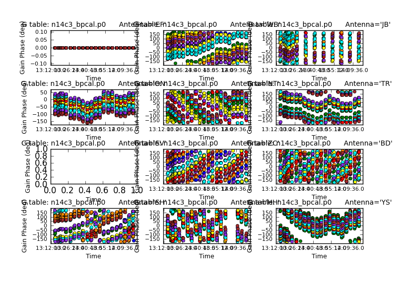
For each spw, in a different color, the corrections have a systematic shape. These solutions are also smooth in time which means (normally) that these are ok!
c. Bandpass correction
We use the bandpass calibration source 1848+283 to derive channel-by-channel corrections for phase and amplitude. We apply the phase vs. time calibration table ()n14c3_bpcal.p0) to allow the data to be averaged in time, and we apply the delay and Tsys/gain curve correction tables to provide preliminary per-spw corrections to the slope of the phase and the overall amplitude fluctuations with time.
Since we have not provided a different model, bandpass uses a default 1 Jy model at the phase centre; hence we normalise the amplitude corrections, so there are different corrections as needed per channel but they are normalised by the overall product (over all time on this source but in each spw).
- To do bandpass correction we use the aptly named task
bandpass:
#In CASA

os.system('rm -rf n14c3.B')
default(bandpass)
vis='n14c3.ms'
caltable='n14c3.B'           # output bandpass calibration table
field='1848+283'
solint='inf'
combine='scan'               # average all the data in time
refant='EF'
solnorm=T                    # Keep the product of corrections unity so the flux scale is not changed overall
gaintable=['n14c3_bpcal.K','n14c3_bpcal.p0','n14c3.tsys','n14c3.gc']
interp='nearest'
parang=T

bandpass()
The solutions fail for the end channels we have flagged but the rest are OK.
- Plot the bandpass table.
# In CASA
default(plotcal)

caltable='n14c3.B'
xaxis='freq'
yaxis='phase'
iteration='antenna'
subplot=431

plotcal()

xaxis='freq'
yaxis='amp'
plotcal()
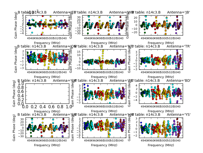
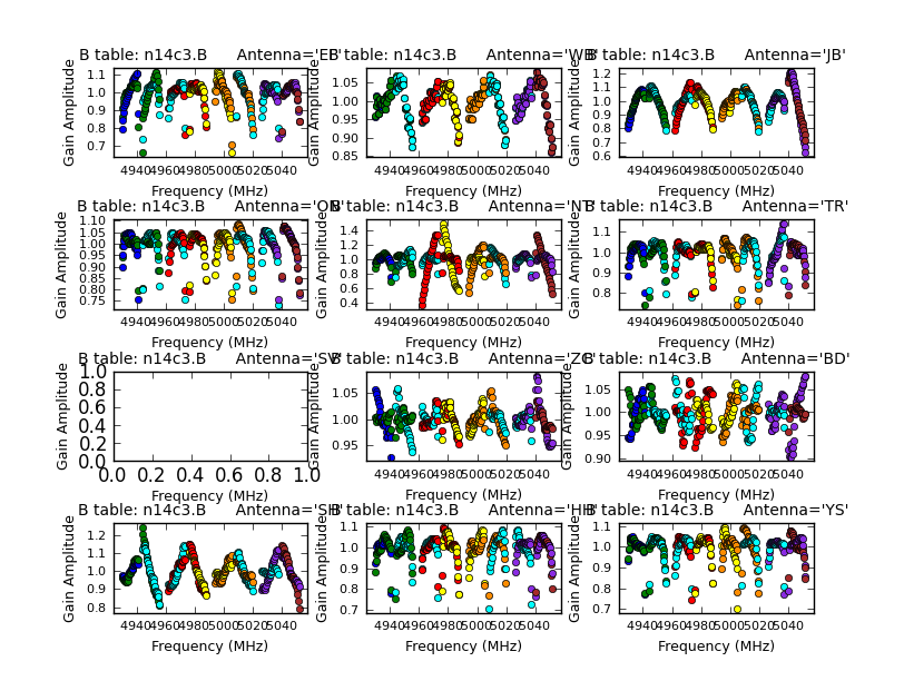
The phase corrections are mostly small, larger close to the remaining end channels, and the amplitude corrections are close to one.
Apply calibration and split out phase-ref - target pairs
Apply the initial calibration
The frequency-dependent calibration i.e. delay, Tsys/gain curve and bandpass, is stable in time over the few hours of these observations and we apply these table to all sources.
Note: we don’t apply the time-dependent phase corrections for the bpcal, because these are not applicable to other sources observed at different times (usually a separate bandpass calibrator is observed before or after the main observations; these are unusual because it is also a phase-cal, but it is convenient to ignore this role here).
- The default mode of
applycalcalibrates the weights (i.e. noisier solutions reduce the weighting given to the data in imaging).
# In CASA
default(applycal)
vis='n14c3.ms'
field=''                      # Apply to all sources
gaintable=['n14c3.tsys','n14c3.gc','n14c3_bpcal.K','n14c3.B']
interp='nearest'
parang=T
applymode='calonly'           # Interpolate or extrapolate over data with missing solutions (don't flag)

applycal()
- And finally we should inspect the corrected data (just one polarisation for simplicity).
default(plotms)
vis='n14c3.ms'
xaxis='freq'
yaxis='amp'
field='1848+283'
ydatacolumn='corrected'   # Applying calibration creates a new 'corrected' data column
correlation='RR'
coloraxis='baseline'
avgtime='3600'
antenna='EF&*'

plotms()

yaxis='phase'
plotms()

xaxis='time'
avgtime=''
avgchannel='32'
plotms()

field=''
coloraxis='field'
yaxis='amp'
plotms()
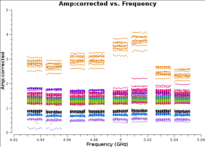
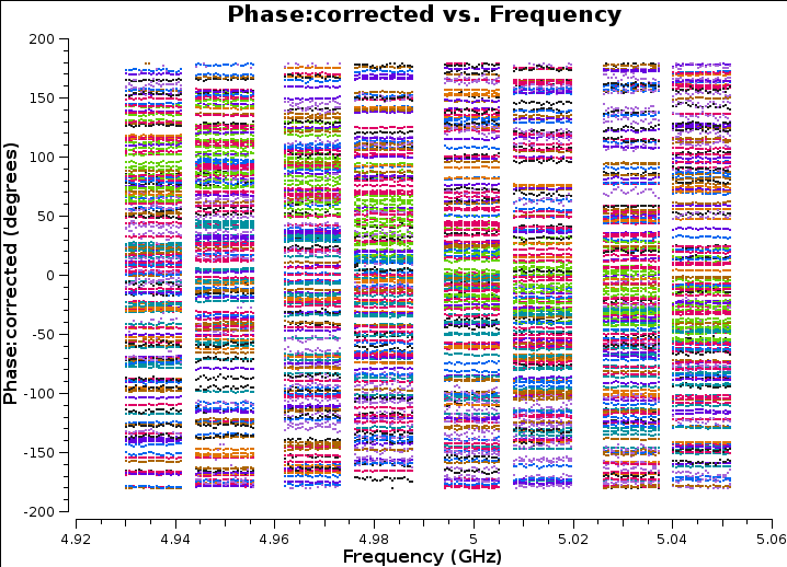
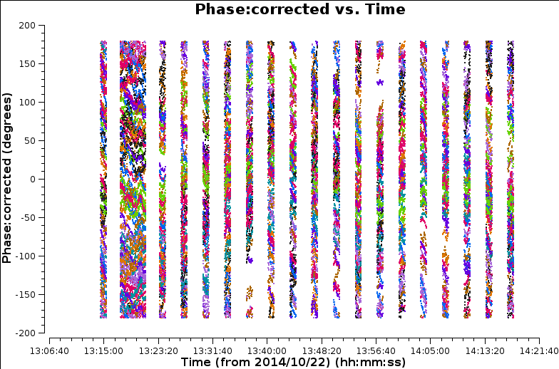
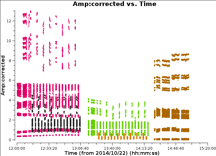
Amplitude and phase are reasonably flat as a function of frequency but different for different antennas and the phase still has a big variation with time, along with some amplitude discrepancies.
Split out each pair of sources
For convenience, split out each phase-reference - target pair separately. The ‘corrected’ column will just be ‘data’ in the newMSs.
We use the task split to do this:
# In CASA
os.system('rm -rf J1640+3946_3C345.ms')
os.system('rm -rf J1640+3946_3C345.ms.flagversions')

default(split)
vis='n14c3.ms'
outputvis='J1640+3946_3C345.ms'
field='J1640+3946,3C345'
datacolumn='corrected'

split()

os.system('rm -rf 1848+283_J1849+3024.ms')
os.system('rm -rf 1848+283_J1849+3024.ms.flagversions')
outputvis='1848+283_J1849+3024.ms'
field='1848+283,J1849+3024'
datacolumn='corrected'

split()
Ignore any ‘file left unfinished’ messages if the lists are OK)
- List each of these
os.system('rm -rf J1640+3946_3C345.ms.listobs')
default(listobs)
vis='J1640+3946_3C345.ms'
listfile='J1640+3946_3C345.ms.listobs'
listobs()

os.system('rm -rf 1848+283_J1849+3024.ms.listobs')
vis='1848+283_J1849+3024.ms'
listfile='1848+283_J1849+3024.ms.listobs'
listobs()
Check the listobs files and go on to the next part CASA_1848+283_J1849+3024. Congratulations this is the end of part 1. This is a scripted example of phase-referencing, imaging and self-calibration.